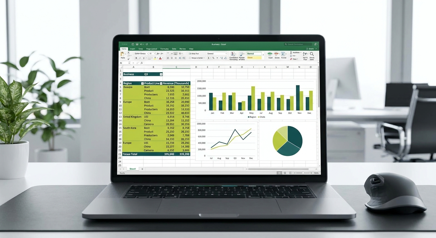
If you have ever opened a spreadsheet full of data and had no idea how to make sense of it, pivot tables are for you. They do not require any data analysis background. You do not need formulas, coding, or even a deep understanding of Excel. This guide will show you exactly how to get started, step by step.

What Is a Pivot Table, in Plain English?

A pivot table takes a long list of raw data and summarises it into a clean, readable table. Think of it like asking your spreadsheet a question and getting a direct answer.

Here are two common business examples:

• Sales by region: You have 500 rows of sales transactions. A pivot table can instantly show you the total revenue per state, without writing a single formula.
• Expenses by category: Your finance team has logged hundreds of expenses. A pivot table groups them by category (travel, software, marketing) and shows the total for each.

That is the core idea. Raw data in, clear summary out.

How to Create Your First Pivot Table

Follow these steps to create a pivot table from scratch.

1. Open your spreadsheet and make sure your data has column headers in the first row. Each column should have a clear name, such as “Region”, “Sales Amount”, or “Date”.
2. Click anywhere inside your data range. Excel is smart enough to detect the edges of your table automatically.
3. Go to the Insert tab in the ribbon at the top of Excel.
4. Click PivotTable. A dialogue box will appear. Excel will suggest a range based on your data.
5. Choose where to place the pivot table. The default option is a new worksheet, which keeps things tidy. Click OK.

You now have a blank pivot table with a panel on the right called the PivotTable Fields pane. This is where the real work happens.

Dragging Fields: Rows, Columns, Values, and Filters

The right-hand panel shows all your column headers as fields. You drag these fields into four areas:

• Rows: This becomes the left column of your table. Drag “Region” here to list each region as a row.
• Columns: This splits your data horizontally. Drag “Quarter” here to see columns for Q1, Q2, Q3, and Q4.
• Values: This is the number Excel calculates. Drag “Sales Amount” here to see totals.
• Filters: This adds a dropdown at the top of the table. Drag “Product Category” here to filter everything by category with one click.

Start simple. Just Rows and Values is enough to get useful results on your first attempt.

Changing the Calculation: Sum, Count, Average

By default, Excel will sum your Values field. But you can change this easily.

1. Click on the field inside the Values area in the right-hand panel.
2. Select Value Field Settings.
3. Choose from Sum, Count, Average, Max, Min, and others.
4. Click OK.

Count is useful when you want to know how many transactions occurred, rather than the total dollar value. Average works well for things like average deal size or average response time.

How to Refresh a Pivot Table When Your Data Changes

Pivot tables do not update automatically when you add or change data. This is one of the most common frustrations for new users.

To refresh your pivot table:

1. Click anywhere inside the pivot table.
2. Right-click and select Refresh.
3. Alternatively, go to the PivotTable Analyse tab and click Refresh.

If you added new rows below your original data range, you will also need to update the data source. Go to PivotTable Analyse, click Change Data Source, and expand the range to include your new rows.

How to Add a Slicer for Easy Filtering

Slicers are visual filter buttons that sit on top of your spreadsheet. They make filtering fast and intuitive, especially when sharing reports with colleagues who are not Excel-savvy.

1. Click inside your pivot table.
2. Go to the PivotTable Analyse tab.
3. Click Insert Slicer.
4. Tick the fields you want to filter by, such as “Region” or “Product Category”.
5. Click OK.

You will now see buttons for each unique value in that field. Click a button to filter the pivot table instantly. Click it again to remove the filter. Hold Ctrl to select multiple values at once.

How Copilot in Excel Removes the Barrier

If you are on Microsoft 365 with Copilot enabled, you can skip several of the steps above entirely. Copilot lets you describe what you want in plain English, and it builds the pivot table for you.

Here are some example prompts you can use directly in Excel:

• “Show me total sales by product category.”
• “Summarise expenses by department for this quarter.”
• “Which region had the highest average order value last month?”
• “Create a pivot table showing headcount by team and location.”

To use Copilot in Excel, click the Copilot button in the Home tab (it looks like a small sparkle icon). Type your question in the chat panel that appears on the right. Copilot will analyse your data and either build the pivot table for you or walk you through the steps.

This is genuinely useful for people who know what they want to see but are unsure how to set it up. You can also ask Copilot to explain an existing pivot table or suggest insights from your data.

Common Mistakes and How to Avoid Them

• Missing column headers: Your data must have a header row. Without it, Excel cannot build the Fields pane correctly. Always name your columns.
• Blank rows in the middle of your data: These confuse Excel’s auto-detect. Remove any blank rows before creating the pivot table.
• Numbers stored as text: If your Values field shows a count of zero or strange results, check that the column is formatted as a number, not text. Select the column, go to the Data tab, and click Text to Columns to convert it.
• Forgetting to refresh: After updating your source data, always refresh the pivot table. It is easy to present outdated figures without realising it.
• Overcomplicating it early: Start with one Row field and one Value field. Add complexity only once you understand the basics.

Ready to Get More From Your Microsoft 365 Tools?

Pivot tables are just one of the tools inside Microsoft 365 that most businesses are not using to their full potential. If you want to explore how your team could work smarter with the tools you already pay for, we can help.

Book a free consultation with the Otto IT team and we will show you what is possible.

Frequently Asked Questions

Do I need to know Excel formulas to use pivot tables?

No, you do not need any formula knowledge. Pivot tables work entirely through drag and drop, and Microsoft Copilot can build them for you using plain English instructions.

Can I use pivot tables in Google Sheets?

Yes, Google Sheets has a similar feature called Pivot Tables. The interface is slightly different but the core concept is identical.

How do I stop a pivot table from grouping dates automatically?

Right-click on a date field inside the pivot table and select Ungroup. Excel sometimes groups dates into months or years automatically, which can be confusing when you want individual dates.

What if my pivot table shows blank values?

This usually means there is missing data in your source table for that combination of row and column. You can replace blanks with zeros by right-clicking the pivot table, selecting PivotTable Options, and entering 0 in the “For empty cells show” field.

Is Copilot available in all versions of Excel?

Copilot in Excel is available on Microsoft 365 Business Standard, Business Premium, and enterprise plans with the Copilot licence add-on. It is not available in standalone Excel 2019 or 2021 purchases.